Learning Machine Learning: Introduction and Linear Regression
In an earlier post, I had talked about how I went about learning about machine learning and deep learning (ML/DL), and said that I would write brief summaries of the introductory ML/DL concepts I learned during that process. I will do part 1 now, otherwise soon I will start to find the introductory concepts obvious and trivial (which they are not). So for all it is worth, and mostly to keep my brain organized, here is the first post on the introductory ML/DL concepts.
In supervised learning, there is a training phase where a supervisor trains the algorithm with examples of how the output relates to the input. Two basic examples of supervised learning are regression, which uses a continuous extrapolation function for output prediction, and classification, which outputs a classification into buckets/groups. The rest of this post delves into supervised learning via regression. Supervised learning via classification will be the topic of my next learning machine learning post.
(Here is a brief word on unsupervised learning for completeness sake. Unsupervised learning does not have a supervised training phase using labeled training data. Even without any labeled training data to compare the output with, we can still do useful work: we can learn some relations among the input data and classify/cluster the input data into groups. So clustering algorithms are a basic example of unsupervised learning category. I won't be mentioning unsupervised learning for the rest of the post, and probably a good while in the future.)
In the rest of this post, I follow/summarize from Andrew Ng's machine learning course at Coursera. (Here is Ng's course material for CS 229 at Stanford.) There are also good course notes here, and I summarize even more briefly than those notes to highlight the big ideas.
This is how linear regression works. The algorithm outputs a function: hypothesis, denoted as h. For example, $h= \theta_0 + \theta_1 * x$. The output, y, is given by h(x), which is a linear function of x, the input. The parameters $\theta_0$ and $\theta_1$ are calculated by the linear regression algorithm using gradient descent.
To calculate $\theta_0$ and $\theta_1$, linear regression uses the cost function approach. To this end, we rewrite the problem as a minimization of error/cost problem. We define cost "$J$" as $(h_θ (x)-y)^2$, and figure out which assignment to θ (i.e., $\theta_0$ and $\theta_1$, also known as the model parameters) gives the minimum error/cost for the training data. $J (θ_0, θ_1) = 1/2m * \sum_{i=1}^m (h_θ (x_i)-y_i)^2$

More specifically, we look at the slope of the cost function and descend the gradient with step sizes of $\alpha$. Iterating like this, we eventually(?) hit a local minima, which for a convex cost function/shape is also the global minima.
More concretely, to compute $\theta_0, \theta_1$ that minimizes cost function $J (\theta_0, \theta_1)$, we do the following until convergence: $\theta_j = \theta_j - \alpha \frac{\partial}{\partial \theta_j} J (\theta_0, \theta_1)$.
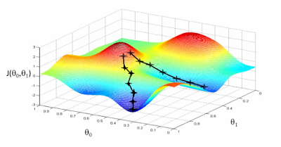
Here is an example with $\theta_0, \theta_1$. The cost function $J$ is a circle/oval. (If there were only $\theta_1$, $J$ would be a line. If there were $\theta_k$, for $k>3$, $J$ would be hard to draw.)

Here $\alpha$ is the learning rate. While calculating $\theta_j$, we update simultaneously for $\theta_0$ and $\theta_1$.

Too small an $\alpha$ would mean that convergence takes a long time. Too big an $\alpha$ may lead to missing convergence and even divergence. To set a suitable value for $\alpha$, we can explore and identify an $\alpha$ that is good enough. To do this we can try a range of alpha values 0.001, 0.003, 0.01, 0.03. 0.1, 0.3, and plot $J(\theta)$ vs number of iterations for each version of $\alpha$. What can I say, ML is a very empirical field of study.

If you have a problem with multiple features, you should make sure those features have a similar scale. If not, the circle (or more accurately the multidimensional spherical shape) could be dominated by one feature $\theta_j$, and would have a very slanted/elongated oval shape rather than a nice circle. And that will prevent the gradient descent to converge quickly to the eye of the target as it will spend too much time walking through the elongated oval.
For feature scaling we can employ mean normalization: Take a feature $x_i$, Replace it by ($x_i$ - mean)/max. Now your values all have an average of about 0.
Supervised and Unsupervised Learning Algorithms
Machine learning algorithms are divided broadly into two parts: supervised and unsupervised learning algorithms.In supervised learning, there is a training phase where a supervisor trains the algorithm with examples of how the output relates to the input. Two basic examples of supervised learning are regression, which uses a continuous extrapolation function for output prediction, and classification, which outputs a classification into buckets/groups. The rest of this post delves into supervised learning via regression. Supervised learning via classification will be the topic of my next learning machine learning post.
(Here is a brief word on unsupervised learning for completeness sake. Unsupervised learning does not have a supervised training phase using labeled training data. Even without any labeled training data to compare the output with, we can still do useful work: we can learn some relations among the input data and classify/cluster the input data into groups. So clustering algorithms are a basic example of unsupervised learning category. I won't be mentioning unsupervised learning for the rest of the post, and probably a good while in the future.)
In the rest of this post, I follow/summarize from Andrew Ng's machine learning course at Coursera. (Here is Ng's course material for CS 229 at Stanford.) There are also good course notes here, and I summarize even more briefly than those notes to highlight the big ideas.
Linear Regression
Linear regression is a basic supervised learning problem for regression. A canonical application for linear regression is learning house pricing via using existing house pricing data by inferring how the sales price of the houses relates to the number of rooms, square-footage, and the location of the houses.This is how linear regression works. The algorithm outputs a function: hypothesis, denoted as h. For example, $h= \theta_0 + \theta_1 * x$. The output, y, is given by h(x), which is a linear function of x, the input. The parameters $\theta_0$ and $\theta_1$ are calculated by the linear regression algorithm using gradient descent.
To calculate $\theta_0$ and $\theta_1$, linear regression uses the cost function approach. To this end, we rewrite the problem as a minimization of error/cost problem. We define cost "$J$" as $(h_θ (x)-y)^2$, and figure out which assignment to θ (i.e., $\theta_0$ and $\theta_1$, also known as the model parameters) gives the minimum error/cost for the training data. $J (θ_0, θ_1) = 1/2m * \sum_{i=1}^m (h_θ (x_i)-y_i)^2$
Gradient Descent
OK, now that we have the cost function $J(\theta_0, \theta_1)$, how do we go about calculating the $\theta$ parameters that minimize the error/cost for the training data? What technique do we use? We let the error/cost function (also known as "loss") be our guide, and perform a locally (myopically) guided walk in the parameter space towards the direction where the error/cost function is reduced. In other words, we descent on the gradient of the error/cost function.
More specifically, we look at the slope of the cost function and descend the gradient with step sizes of $\alpha$. Iterating like this, we eventually(?) hit a local minima, which for a convex cost function/shape is also the global minima.
More concretely, to compute $\theta_0, \theta_1$ that minimizes cost function $J (\theta_0, \theta_1)$, we do the following until convergence: $\theta_j = \theta_j - \alpha \frac{\partial}{\partial \theta_j} J (\theta_0, \theta_1)$.
Here is an example with $\theta_0, \theta_1$. The cost function $J$ is a circle/oval. (If there were only $\theta_1$, $J$ would be a line. If there were $\theta_k$, for $k>3$, $J$ would be hard to draw.)

Here $\alpha$ is the learning rate. While calculating $\theta_j$, we update simultaneously for $\theta_0$ and $\theta_1$.

Too small an $\alpha$ would mean that convergence takes a long time. Too big an $\alpha$ may lead to missing convergence and even divergence. To set a suitable value for $\alpha$, we can explore and identify an $\alpha$ that is good enough. To do this we can try a range of alpha values 0.001, 0.003, 0.01, 0.03. 0.1, 0.3, and plot $J(\theta)$ vs number of iterations for each version of $\alpha$. What can I say, ML is a very empirical field of study.
Linear regression with multiple features
Lets talk about how to generalize linear regression from the linear regression with 1 feature we considered above. Here we make $\theta$ and $x$ into a vector and the algorithm is the same as that of linear regression. Here is the generalized algorithm:
If you have a problem with multiple features, you should make sure those features have a similar scale. If not, the circle (or more accurately the multidimensional spherical shape) could be dominated by one feature $\theta_j$, and would have a very slanted/elongated oval shape rather than a nice circle. And that will prevent the gradient descent to converge quickly to the eye of the target as it will spend too much time walking through the elongated oval.
For feature scaling we can employ mean normalization: Take a feature $x_i$, Replace it by ($x_i$ - mean)/max. Now your values all have an average of about 0.


Comments