Learning Machine Learning: Logistic Regression
This is part 2 of learning machine learning introductory concepts. Recall that supervised learning had two basic examples, regression and classification. We covered linear regression in part 1, and now in part 2 we look at classification. Although the name of the technique used here, logistic regression, includes the word "regression", this is in fact a classification algorithm. It builds on a similar gradient descent approach as we discussed in part 1 in the context of linear regression.
(In this post, again I follow/summarize from Andrew Ng's machine learning course at Coursera. Here is Ng's course material for CS 229 at Stanford. There are also good course notes here, and I will summarize even more briefly than those notes to highlight only the big ideas.)

For linear regression, our hypothesis representation was of the form $h_\theta(x) = (\theta x)$. For classification, our hypothesis representation is of the form $h_\theta(x) = g((\theta x))$, where we define $g(z)= \frac{1}{(1 + e^{-z})}$. This is known as the sigmoid function, or the logistic function. For a real value $z$, the logistic function has the following plot.

If $z$ is positive, $g(z)$ is greater than 0.5. In our logistic regression hypothesis, we take $z = (\theta x)$, so when $\theta x \geq 0$, then $h_\theta \geq 0.5$ and the hypothesis predicts $y=1$. When $\theta x \leq 0$ then the hypothesis predicts $y=0$.
In other words, $\theta x \geq 0$ is the decision boundary. When our hypothesis $h_\theta(x)$ outputs a number, we treat that value as the estimated probability that y=1 on input x.
If our hypothesis is linear, of the form $h_\theta(x) = g(\theta_0 + \theta_1 x_1 + \theta_2 x_2)$, the decision boundary would be a line. For example:

If our hypothesis is polynomial, $h_\theta(x) = g(\theta_0 + \theta_1 x_1 + \theta_2 x_1^2 + \theta_3 x_2^2)$ , the decision boundary can be a circle. (By using higher order polynomial terms, you can get even more complex decision boundaries.) For example:

OK, assuming we had decided on our hypothesis, how does the logistic regression algorithm learn values for fitting $\theta$ to the data to capture the data nicely in the decision boundary? We again use gradient descent, but this time a little differently as follows.
We define our cost function as:

Note that:
cost (1)= 0 if y=1, else it is infinity
cost (0)=0 if y=0, else it is infinity
In other words, this cost function harshly penalizes and thus aims to rule out very confident mislabels; mislabels can still have lukewarm 0.6 confidence because the penalty is less there.
The above is the cost for a single example. For binary classification problems y is always 0 or 1, and using this, we can have a simpler way to write the cost function, and compress it into one equation as follows.

where $\frac{\partial}{\partial \theta_j} J(\theta)= \sum_{i=1}^m (h_\theta (x^i)-y^i)*x_j^i$.

(In this post, again I follow/summarize from Andrew Ng's machine learning course at Coursera. Here is Ng's course material for CS 229 at Stanford. There are also good course notes here, and I will summarize even more briefly than those notes to highlight only the big ideas.)
Hypothesis representation
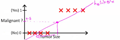
The goal of the logistic regression algorithm is to determine what class a new input should fall into. Here is an example application. See, line fitting does not make sense for this application. We need discrete classification into yes or no categories.
For linear regression, our hypothesis representation was of the form $h_\theta(x) = (\theta x)$. For classification, our hypothesis representation is of the form $h_\theta(x) = g((\theta x))$, where we define $g(z)= \frac{1}{(1 + e^{-z})}$. This is known as the sigmoid function, or the logistic function. For a real value $z$, the logistic function has the following plot.

If $z$ is positive, $g(z)$ is greater than 0.5. In our logistic regression hypothesis, we take $z = (\theta x)$, so when $\theta x \geq 0$, then $h_\theta \geq 0.5$ and the hypothesis predicts $y=1$. When $\theta x \leq 0$ then the hypothesis predicts $y=0$.
In other words, $\theta x \geq 0$ is the decision boundary. When our hypothesis $h_\theta(x)$ outputs a number, we treat that value as the estimated probability that y=1 on input x.
If our hypothesis is linear, of the form $h_\theta(x) = g(\theta_0 + \theta_1 x_1 + \theta_2 x_2)$, the decision boundary would be a line. For example:

If our hypothesis is polynomial, $h_\theta(x) = g(\theta_0 + \theta_1 x_1 + \theta_2 x_1^2 + \theta_3 x_2^2)$ , the decision boundary can be a circle. (By using higher order polynomial terms, you can get even more complex decision boundaries.) For example:

OK, assuming we had decided on our hypothesis, how does the logistic regression algorithm learn values for fitting $\theta$ to the data to capture the data nicely in the decision boundary? We again use gradient descent, but this time a little differently as follows.
Cost function for logistic regression
Since $h_\theta(x) = h_\theta(\frac{1}{(1 + e^{-x})})$ is a sigmoid/nonlinear function, when we plug this in the cost function, we don't know if the cost function will be convex or not. However, the cost function should be convex for the gradient descent to work. So we use a trick, we define our cost function carefully to make sure when $h_\theta(\frac{1}{(1 + e^{-x})})$ is plugged in the cost function, the function is still a convex function.We define our cost function as:
Note that:
cost (1)= 0 if y=1, else it is infinity
cost (0)=0 if y=0, else it is infinity
In other words, this cost function harshly penalizes and thus aims to rule out very confident mislabels; mislabels can still have lukewarm 0.6 confidence because the penalty is less there.
The above is the cost for a single example. For binary classification problems y is always 0 or 1, and using this, we can have a simpler way to write the cost function, and compress it into one equation as follows.
Gradient descent for logistic regression
We use gradient descent to minimize the logistic regression cost function. As described before the gradient descent algorithm repeatedly does the following update $\theta_j := \theta_j - \alpha \frac{\partial}{\partial \theta_j} J(\theta)$,where $\frac{\partial}{\partial \theta_j} J(\theta)= \sum_{i=1}^m (h_\theta (x^i)-y^i)*x_j^i$.
Multiclass classification problems
We can adopt this singleclass logistic regression idea for solving a multiclass classification problem using one vs. all approach: To do k classifications, split the training set into k separate binary classification problems.


Comments