Paper Summary: Two decades of recommender systems at Amazon.com
This is a short article that appeared as a retrospective piece for the 2003 "Item-to-Item Collaborative filtering" paper as it was awarded a test-of-time award. This article is by Brent Smith and Greg Linden.
I am not a machine-learning/data-mining guy, so initially I was worried I wouldn't understand or enjoy the article. But this was a very fun article to read, so I am writing a summary.
The item-based collaborative filtering is an elegant algorithm that changed the landscape of collaborative filtering which was user-based till then. User-based means "first search across other users to find people with similar interests (such as similar purchase patterns), then look at what items those similar users found that you haven't found yet". Item-based is based on the idea that "people who buy one item are unusually likely to buy the other." So, for every item i1, we want every item i2 that was purchased with unusually high frequency by people who bought i1.
The beauty of the approach is most of the computation is done offline. Once the related items table is built, we can generate recommendations quickly as a series of lookups. Moreover since the number of items sold is less than the users, this scales to better user numbers.
This was implemented for Amazon.com for recommending related products (mostly books at that time). Since 2003, item-based collaborative filtering has been adopted by YouTube and Netflix, among others.
To define related, we should define what it means for Y to be unusually-likely to be bought by X buyers. And for figuring this out, we should first figure out the reverse, what is the expected ratio that X buyers would buy Y if the two items were unrelated.
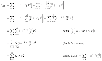
The straightforward way to estimate the number of customers, Nxy, who have bought both X and Y would be to assume X buyers had the same probability, P(Y) = |Y_buyers|/|all_buyers|, of buying Y as the general population and use |X_buyers| * P(Y) as the estimate, Exy, of the expected number of customers who bought both X and Y. In fact, the original 2003 algorithm had used this ratio.
But this ratio is misleading, because for almost any two items X and Y, customers who bought X will be much more likely to buy Y than the general population. "Heavy buyers" are to blame for this situation. We have a biased sample. For any item X, customers who bought X (this set has many heavy buyers in it by definition) will be likely to have bought Y more than the general population.
Figure 1 shows how to account for this effect.

Now, knowing Exy, we can use it to evaluate whether Nxy, the observed number of customers who bought both X and Y, is higher or lower than randomly would be expected. For example, Nxy-Exy gives an estimate of the number of non-random cooccurrences, and [Nxy-Exy]/Exy gives the percent difference from the expected random co-occurrence.
In another surprise, neither of those work quite well. The first will be biased towards popular Ys, and the second makes it to easy for low-selling items to have high scores. The chi-square score, $[Nxy−Exy]/\sqrt{Exy}$ strikes the balance.
Worth noting was the observation that some items have more weight. They found that a single book purchase can say a lot about a customer's interests than an arbitrary product, letting them recommend dozens of highly relevant items.
For the future, the article envisions intelligent interactive services where shopping is as easy as a conversation, and the recommender system knows you as well as your spouse or a close friend.
I am not a machine-learning/data-mining guy, so initially I was worried I wouldn't understand or enjoy the article. But this was a very fun article to read, so I am writing a summary.
The item-based collaborative filtering is an elegant algorithm that changed the landscape of collaborative filtering which was user-based till then. User-based means "first search across other users to find people with similar interests (such as similar purchase patterns), then look at what items those similar users found that you haven't found yet". Item-based is based on the idea that "people who buy one item are unusually likely to buy the other." So, for every item i1, we want every item i2 that was purchased with unusually high frequency by people who bought i1.
The beauty of the approach is most of the computation is done offline. Once the related items table is built, we can generate recommendations quickly as a series of lookups. Moreover since the number of items sold is less than the users, this scales to better user numbers.
This was implemented for Amazon.com for recommending related products (mostly books at that time). Since 2003, item-based collaborative filtering has been adopted by YouTube and Netflix, among others.
Defining related items
This section was tricky and fun. Statistics is not a very intuitive area. At least for me. While reading this section I saw proposals to fix things, and thought they would work, and I was wrong. Twice.To define related, we should define what it means for Y to be unusually-likely to be bought by X buyers. And for figuring this out, we should first figure out the reverse, what is the expected ratio that X buyers would buy Y if the two items were unrelated.
The straightforward way to estimate the number of customers, Nxy, who have bought both X and Y would be to assume X buyers had the same probability, P(Y) = |Y_buyers|/|all_buyers|, of buying Y as the general population and use |X_buyers| * P(Y) as the estimate, Exy, of the expected number of customers who bought both X and Y. In fact, the original 2003 algorithm had used this ratio.
But this ratio is misleading, because for almost any two items X and Y, customers who bought X will be much more likely to buy Y than the general population. "Heavy buyers" are to blame for this situation. We have a biased sample. For any item X, customers who bought X (this set has many heavy buyers in it by definition) will be likely to have bought Y more than the general population.
Figure 1 shows how to account for this effect.

Now, knowing Exy, we can use it to evaluate whether Nxy, the observed number of customers who bought both X and Y, is higher or lower than randomly would be expected. For example, Nxy-Exy gives an estimate of the number of non-random cooccurrences, and [Nxy-Exy]/Exy gives the percent difference from the expected random co-occurrence.
In another surprise, neither of those work quite well. The first will be biased towards popular Ys, and the second makes it to easy for low-selling items to have high scores. The chi-square score, $[Nxy−Exy]/\sqrt{Exy}$ strikes the balance.
Extensions
The article talks about tons of extensions possible. Using the feedback data about user clicks on recommendations, it is possible to further tune the recommender. One should also take into account time of purchases, causality of purchases, compatibility of purchases. One should also account for aging the history and aging the recommendation as the user ages.Worth noting was the observation that some items have more weight. They found that a single book purchase can say a lot about a customer's interests than an arbitrary product, letting them recommend dozens of highly relevant items.
For the future, the article envisions intelligent interactive services where shopping is as easy as a conversation, and the recommender system knows you as well as your spouse or a close friend.


Comments